In this project we explore whether voting patterns of United Nations members reflect political alignments. We use cluster the nations using K-means on data containing historical voting patterns of UN members.

unsupervised learning, clustering and K-means

Unsupervised learning methods have no response variable. The objective is not related to prediction but rather to the identification of different possible structures that may be present in the data. For example, one may be interested in determining whether the observations are grouped in some way (clustering). In this study project we look at clustering nations in the UN.

The objective of clustering can be described as identifying different groups of observations that are closer to each other than to those of the other groups. In general, the number of groups is unknown and needs to be determined from the data.

Probably the most intuitive and easier to explain unsupervised clustering algorithm is K-means. We will use K-means on the UN-votes data. Note that the UN-votes data is strictly categorical so using K-means is a bit weird but it turns out it works okay for this example.

UN votes example

These data contain the historical voting patterns of United Nations members. The data include only “important” votes, as classified by the U.S. State Department. The votes for each country were coded as follows: Yes (1), Abstain (2), No (3), Absent (8), Not a Member (9). There were 368 important votes, and 77 countries voted in at least 95% of these. We focus on these UN members.

Lets explore whether voting patterns reflect political alignments, and also whether countries vote along known political blocks. Our data consists of 77 observations with 368 variables each.

We read in the data, and limit ourselves to resolutions where every country voted without missing votes:

X <- read.table(file='unvotes.csv', sep=',', row.names=1, header=TRUE)
X2 <- X[complete.cases(X),]

We now compute a K-means partition with K = 5, and look at the resulting groups:

set.seed(123)
b <- kmeans(t(X2), centers=5, iter.max=20, nstart=1)
table(b$cluster)

## 
##  1  2  3  4  5 
## 18  2  7 19 31

Note that if we run K-means again, we might get a different partition:

b <- kmeans(t(X2), centers=5, iter.max=20, nstart=1)
table(b$cluster)

## 
##  1  2  3  4  5 
## 27 12 13  7 18

This is because K-means is not a determinisitic algorithm and the final clusterings it chooses will depend on an initial random seed. To avoid clusterings that result from an “unlucky” seed, it is better to consider a large number of random starts and take the best found solution.

# Take the best solution out of 1000 random starts
b <- kmeans(t(X2), centers = 5, iter.max = 20, nstart = 1000)
split(colnames(X2), b$cluster)

## $`1`
##  [1] "Argentina"  "Bahamas"    "Brazil"     "Chile"      "Colombia"  
##  [6] "Costa.Rica" "Mexico"     "Panama"     "Paraguay"   "Peru"      
## [11] "Uruguay"   
## 
## $`2`
## [1] "Israel" "USA"   
## 
## $`3`
##  [1] "Bolivia"             "Botswana"            "Burkina.Faso"       
##  [4] "Ecuador"             "Ethiopia"            "Ghana"              
##  [7] "Guyana"              "Jamaica"             "Jordan"             
## [10] "Kenya"               "Mali"                "Nepal"              
## [13] "Nigeria"             "Philippines"         "Singapore"          
## [16] "Sri.Lanka"           "Tanzania"            "Thailand"           
## [19] "Togo"                "Trinidad.and.Tobago" "Zambia"             
## 
## $`4`
##  [1] "Algeria"              "Bangladesh"           "Belarus"             
##  [4] "Brunei.Darussalam"    "China"                "Cuba"                
##  [7] "Egypt"                "India"                "Indonesia"           
## [10] "Kuwait"               "Libya"                "Malaysia"            
## [13] "Pakistan"             "Russian.Federation"   "Sudan"               
## [16] "Syrian.Arab.Republic" "Venezuela"           
## 
## $`5`
##  [1] "Australia"   "Austria"     "Belgium"     "Bulgaria"    "Canada"     
##  [6] "Cyprus"      "Denmark"     "Finland"     "France"      "Greece"     
## [11] "Hungary"     "Iceland"     "Ireland"     "Italy"       "Japan"      
## [16] "Luxembourg"  "Malta"       "Netherlands" "New.Zealand" "Norway"     
## [21] "Poland"      "Portugal"    "Spain"       "Sweden"      "UK"         
## [26] "Ukraine"

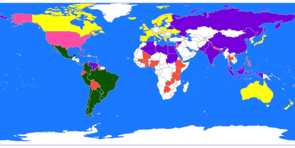
Lets view the clustering on a map:

library(rworldmap)
library(countrycode)
these <- countrycode(colnames(X2), "country.name", "iso3c")
malDF <- data.frame(country = these, cluster = b$cluster)
malMap <- joinCountryData2Map(malDF, joinCode = "ISO3", nameJoinColumn = "country")

par(mai = c(0, 0, 0, 0), xaxs = "i", yaxs = "i")
mapCountryData(malMap, nameColumnToPlot = "cluster", catMethod = "categorical", 
    missingCountryCol = "white", addLegend = FALSE, mapTitle = "", colourPalette = c("darkgreen", 
        "hotpink", "tomato", "blueviolet", "yellow"), oceanCol = "dodgerblue")

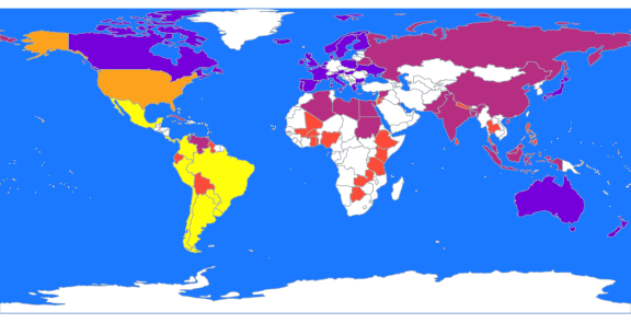
Now we use K-means with K=3 to obtain clusters that may be easier to interpret:

library(cluster)
these <- countrycode(colnames(X2), "country.name", "iso3c")
malDF <- data.frame(country = these, cluster = b$cluster)
malMap <- joinCountryData2Map(malDF, joinCode = "ISO3", nameJoinColumn = "country")

par(mai = c(0, 0, 0, 0), xaxs = "i", yaxs = "i")
mapCountryData(malMap, nameColumnToPlot = "cluster", catMethod = "categorical", 
    missingCountryCol = "white", addLegend = FALSE, mapTitle = "", colourPalette = c("yellow", 
        "tomato", "blueviolet"), oceanCol = "dodgerblue")

authors

• Evan James Martin